Mathematical Computations

Updated 11/19/21

This section isn't for everyone, and is not essential to your use of FastTrack, but tech support is often asked to explain . . . so here is the explanation.

AccuTrack
Adjusted Return (J & 2 Charts)
Annualized Total Return (CAGR) (Ann=)
Family Average (AVG)
Beta
Bollinger Bands
Correlation (Cor=)
Distribution Adjusted Indexes
Distribution Adjusted Prices 
FTAlpha
MACD
Moving Average Computation
Moving Average (V Chart)
NCAlpha (Spreadsheet Column)
Price Chart (P Chart)

Purple Values
Purple Values Relative Standard Deviation
Relative Strength (R Chart
Relevant Index
Risk-Free Return
Rr= Risk return (J and 2 Charts)
Sharpe Ratio
Standard Deviation (SD=
Stochastics (S Chart
Total Return
Ulcer Index
Ulcer Performance Index (UPI
Welles Wilder RSI (I Chart)
Weird Numbers
Yellow Values
Yield on the spreadsheet
Yield1Y: Yield One Year (SEC mandated)

Moving Averages in General and the V Chart

The Moving Average indicator has one adjustable parameter. FastTrack uses the exponential moving average. All moving averages within FastTrack are calculated using an exponential average. For a simple formula for exponential moving average, click here.

1. The calculation uses a smoothing factor derived from the first Moving Average parameter.

SFactor=2/(1stParameter + 1)

2. Each day's moving average value is computed as follows,

MA=(Price*SFactor)+(MA*(1- SFactor))

3. When the 2nd Moving average parameter is 1 or greater then, the above process is repeated using the 2nd parameter and computed against the already averaged daily values instead of the Price.
4. When the 2nd Moving Average parameter is taken as a percentage (.05=5%), signals are only generated when the issue and the average differ by the parameter percentage. Also, the plot of the bars is modified to stay appropriately above or below the centerline as required by the filter.
5. On the first day MA is set to the first day's Price. The MA is carried forward to the next day to be used as the MA in the formula. FastTrack plots the difference between the MA and the issue as vertical bars originating at the centerline. When the bars are below the centerline, then the moving average is above the issue line.

Distribution Adjusted Prices

Historical prices must be adjusted for the distributions to reflect an accurate picture of the issue performance over time. FastTrack computations reinvest distributions at the closing price on the x-dividend day. All historical prices from the day before the x-dividend date are reduced backward in time.

When a split occurs, Prices are reduced by the split ratio. For example, when 3-for-1 split occurs, Prices before the x-dividend date will be multiplied by 1/3. A 1-for-5 reverse split is handled the same way: Prices before the x-dividend date will be multiplied by 5.

When the distribution is shares of stock in another company (AT&T spun off Lucent). The value of the new shares at the earliest moment they could have been sold is reinvested in the parent (AT&T).

To compute distribution-adjusted data for yourself. See the Distributions Adjustment WorkSheet.

Distribution-Adjusted Indexes

FastTrack provides a number of dividend adjusted indexes computed by sponsors (S&P, Dow Jones, etc.). There is no standard way that sponsors compute dividend adjusted indexes.  Sources differ. However, our returns are very, very close to other sources.

The index sponsor's daily adjustment is usually based on the prior quarter's dividend rate. Once the most recent quarter's dividend rate is reported, the sponsor recomputes the index for that quarter. When we receive notice of the recomputation, FastTrack reloads the sponsor's index. All changes are sent to subscribers with the regular evening update.

For example

The SP-DA (S&P 500 div-adjusted) is calculated by S&P as follows:
When  the prior quarter's actual dividend is reported, S&P computes a daily adjustment by dividing that the dividend by 63.25 (63.25 is the average number of trading days in a quarter). In the current quarter, each trading day's SP-CP change  (S&P 500 unadjusted as reported in The Wall Street Journal each day) is increased by the daily adjustment. The revised rate is applied the to the prior quarter's close of  SP-DA to produce the revised prices for the quarter.

For those whose work is disturbed by this process, we recommend that they follow the Vanguard S&P 500 fund, VFINX, as a source for real-time dividend adjusted prices which are not subject to quarterly revision.

Indicator and Chart Computations

The computations are described in general fashion below. Not all aspects of the computation are described in detail.

AccuTrack Histogram Indicator (A Chart)

AccuTrack Parameter 1 is a smoothing factor. Parameter 2 governs the length of the moving averages used internally in the computation of AccuTrack. To compute each day's AccuTrack bar:

1. Compute a daily change for the issue and the index by the formula:
     Change= (TodayPrice - YesterdayPrice)/YesterdayPrice

2. Exponentially smooth Change of the red and green lines by Parameter 2 days starting from the 1st date in the database. 

3. Subtract the smoothed Red Line Change and Green Line Change computed above.
     Diff= Red Line Change - Green Line Change
4. Exponentially smooth Diff by Parameter 1.
5. Check the data for the maximum and minimum values. Then scale the data to fit in the range -100 to +100 range. The computation is based on the greatest high or low absolute value. This means that only the positive side or the negative will actually reach the +/-100 value.
6. Plot each day's value as a vertical bar with 0 falling at the centerline.

Annualized Return (Ann=)

The calculation is performed in the following equation:

  ((TotalReturn + 1 ) ^ ( 252.25  / MarketDays ) - 1

• TotalReturn
  The total return calculated for the period using distribution-adjusted data.
  Total return is calculated as per the Distributions Adjustment Worksheet.
• MarketDays
   A count of days over which the TotalReturn was achieved
• 252.25
  The number of market days in a year. Due to market closure September 11-16, 2001, FT's use of this fixed constant will create slight distortions of annualized return over this period.

Note: This calculation is known in the investment industry as Compound Annual Growth Rate (CAGR). There is another calculation called Average Annual Return which takes the return each year and produces and average of the annual return. This is a highly misleading number and IS NOT provided or used by FT4web.

 See Weird Numbers below.

Beta (Bet=)

The algorithm used to compute FastTrack’s Beta was published in “Guide to Portfolio Management”, James L. Farrell, Jr., McGraw-Hill - 1983, pages 41-43.

Beta = (Correlation x issue’s SD)/GreenLine SD

The correlation calculation is ALWAYS done with respect to the green line.

There are a number of different ways to compute Beta so do not expect FastTrack’s method to compute exactly the Beta you might see in some publications.

For Beta to have ANY validity, the red line and the green line MUST be closely correlated (having a Cor= value of 0.95 or higher). Beta reports a NA value when less than 15 market days are used

Bollinger Bands (B Chart)

The Bollinger Band Chart is a type of Envelope developed by John Bollinger. But instead of plotting the envelope at a fixed percentage from the moving average, the Upper and Lower bands are plotted at Standard Deviation levels above and below the moving average.

Because standard deviation is a measure of volatility, Bollinger bands adjust themselves to the market conditions. When the markets become more volatile the bands widen (move further away from the average), and, during less volatile periods, the bands contract (move closer to the average).

The Bollinger Band Chart has two adjustable parameters, P (period of the Simple Moving Average) and D (the number of Standard Deviations to shift the upper and lower bands).

Bollinger Calculation

1. Calculate a Simple Moving Average of length P of the selected Fund.
2. Calculate the Standard Deviation of the Simple Average (from Step 1) from selected Fund.
3. For all days shift Upper and Lower bands according to that day's Standard Deviation
4. Upper Band [Day] = Simple Moving Average [Day] + Standard Deviation [Day]
5. Lower Band [Day] = Simple Moving Average [Day] - Standard Deviation [Day]; 

FTAlpha

We do not disclose the mathematics for this indicator. FTAlpha is the sole proprietary formula within FastTrack.

FTAlpha combines correlation, risk, and return. The computations for the spreadsheet FTAlpha column compare an issue to the Low Risk Basis for the correlation portion of the computation. When computing an AVG using FTAlpha, the AVG currently being computed is used instead of using the Low Risk Basis.

Correlation (Link to general discussion

MACD Indicator (M Chart)

The MACD indicator has three adjustable parameters, P1(length of slow moving average), P2 (length of fast moving average), and P3 (length of trigger moving average). It is calculated using only the red line. The steps in charting the indicator are as follows:

1. Compute a slow exponential moving average of the issue using P1. In general, P1 must be greater than P2.
2. Compute a fast exponential average of the issue using P2

3. Subtract the Fast Average from the Slow Average for each day. The difference is the MACD Value. 
   
   Slow-Fast = MACD Value

4. Calculate an exponential average of the MACD Values using P3. These are the trigger values.
   
   ExponentialAverage^P3(MACD Values) = Trigger line
    

5. Subtract the MACD Values from the trigger values.
   
   Trigger values-MACD Values = MACD histogram values
    

6. Check the data for the maximum and minimum values. Then scale the data to fit in the range -100 to +100 range. The  computation is based on the absolute value of greater of  high and low . This means that only the positive side or the negative will actually reach the +/-100 value.

7. Plot each day's MACD histogram value as a vertical bar with 0 falling at the centerline. Plot positive and negative values  as bars originating from the centerline.

Moving Average Histogram Indicator (V Chart)

This indicator's calculations are done on the red line only.

1. The indicator has two parameters. First, calculate two exponential moving averages using the parameters.
2. Compute the differences (Subtract) between the moving averages each day
3. Check the data for the maximum and minimum values. Then scale the data to fit in the range -100 to +100 range. The computation is based on the greatest high or low absolute value. This means that only the positive side or the negative will actually reach the +/-100 value.
4. Plot each day's value as a vertical bar with 0 falling at the centerline.

Click for more information about Moving Average compared to the P and M Charts.

NC Alpha

This calculation measures the excess return of an issue with respect to the low risk basis. Issues with more return per unit of volatility than the low risk basis line have positive NCAlpha values. Issues with less return per unit of volatility have negative NCAlpha values. The formula is,

NCAlpha = XTotReturn! - (Low Risk Basis Return! * XSD! / Low Risk Basis SD!)

Where . . .

• XTotReturn is the total return of any given issue for the period of the currently displayed chart.

• Click for the definition of the Low Risk Basis

• XSD is the the given issue's Standard Deviation for the chart period.

• SD of the Low Risk Basis for the chart period.

P Chart

The red line is a plot of Adjusted Price. The yellow and purple lines are exponential moving averages of the Adjusted Price. The values reported by the Dashed Pole are based on the reported (i.e. not adjusted) price as it appeared in the paper on any given day. The red value is the price as in the paper. The yellow and purple values are the exponential moving averages using the number of yellow or purple days on the screen.

As more data accumulates and more distributions are paid, then the Adjusted Price changes BUT because of the formula given above, the reported yellow and purple values are unchanged.

This means that if you plot the red, yellow, and purple values reported by the Dashed Pole, then the lines would have major discontinuities at each distribution. In the FT chart these discontinuities do not appear because the adjusted values are used in drawing the line. The advantage of using this method is that it is possible to use back issues of The Wall Street Journal to check historical data since the prices shown by the Dashed Pole are computed as they were the day the paper was published and the averages are also shown as if computed the day the paper was published.

Click for more information about the Price chart compared to the M and V Charts.

Relative Strength Chart (R Chart)

Relative strength yellow line is the ratio of the total return of the issue to the total return of the index. The value of each point is plotted as follows:

R = (RedTodayPrice /Red1stPrice) /(GreenTodayPrice / Green1stPrice) * 10

where. . .

• RedTodayPrice = The dividend-adjusted red line CP= price on any given day.
• Red1stPrice = The dividend-adjusted price of the issue on the first day. The first day is the later of the start of the red/green data. It is not related to pole positions or span of the data displayed.
• GreenTodayPrice = The price of the green  line on any given day.
• Green1stPrice = The price of the green line on the first day charted.

The short moving average (blue line) is computed using Short Average value from the Parameter Dialog . The long moving average (purple line) is computed using long Avg parameter.

Relevant Index

The Relevant Index is computed as follows:

For every issue in the fund and stocks databases, we compute  correlation to an index, ETF, or Vanguard open end fund. over the most recent one-year period. We look for the highest absolute value correlation. If there is no match of at least 70% correlation the fund is assigned 0% as the RelIndex.   When the test succeeds, then the Relevant index ticker symbol is encoded in the FastTrack database with the issue which was tested. Correlation to self is always ignored.

The correlation index is helpful in classifying funds.  For example for the year 2008, FMAGX, FCNTX, and VFINX are highly correlated. Yet the RelIndexes assigned  

FMAGX, JKH-X( MidCap Growth)
FCNTX, JKE-X( LargeCap Growth)
VFINX, VV   ( LargeCap)

Suggest subtle differences in the management philosophies

Sharpe Ratio

The Sharpe Ratio is calculated as:

(Issue's Annualized Return - Low Risk Basis's Annualized Return) / (Issue's Monthly Standard Deviation * SQR(12))

The classical Sharpe ratio is computed by using IRX-X as the low risk basis. However, since 1998, FT4Web can use any issue or Yield Index for the Sharpe ratio.  While this approach was FastTrack's original implementation, Franco Modigliani apparently had similar thoughts in 1997. We learned of Modigiliani from a FastTracker in 2011.

From Wikipaedia.com:

"In 1997, Nobel-prize winner Franco Modigliani and his granddaughter, Leah Modigliani, developed the Modigliani Risk-Adjusted Performance measure They originally called it "RAP" (Risk Adjusted Performance). They also defined a related statistic, "RAPA" (presumably, Risk Adjusted Performance Alpha), which was defined as RAP minus the risk-free rate (i.e., it only involved the risk-adjusted return above the risk-free rate). Thus, RAPA was effectively the risk-adjusted excess return. The RAP measure has since become more commonly known as "M2"(because it was developed by the two Modiglianis), but also as the "Modigliani-Modigliani measure" and "M2", for the same reason."

IRX-X, US30-, etc. yield index daily values in the FT database are in annualized return form. For the FT4Web Sharpe calculation that return is converted to daily return then compounded daily. The daily result is used in FT4Web's Sharpe computation for the Low Risk Basis's Annualized Return.

This daily compounding method differs from the original Sharpe calculation which assumed that the risk-free rate stayed the same over the period. Sharpe reworked his formula in 1994 acknowledging rate variation adapts this newer Sharpe Approach.  Note, Sharpe make no mention of using annualized values within his calculation. FastTrack considers the use of annualized values to be of critical importance normalizing the index values. Also FT4Web uses highly accurate daily compounded returns whereas Sharpe describes simple averaged returns.

Risk Free-Return

More on IRX-X : This is the CBOE US T-Bill 13-week Yield index. This is also commonly used as the "risk-free" interest rate. Compare IRX-X to FastTrack's US3M-, US 3-month T-Bill yield. IRX-X became a problematic value in late 2008 when it fell to zero and then for a long time  near zero. Its value in The Wall Street Journal was carried as 0-0.25%. The FastTrack  database carries it as 0.25%

The period of 0% return for IRX-X means that the ratio of risk/return cannot be computed (division by zero). The artificial value of 0.25 was carried by FastTrack to avoid the division by zero, but the Sharpe ratio during this period based on IRX-X had no real meaning.

However, using IRX-X has always been a mediocre choice when trying to select the best fund. Using FastTrack Sharpe with a highly correlated risk/return basis works better than using uniformly IRX-X for all issues. (for example, using VFINX for a basis for computing Sharpe on equity funds.)

Standard Deviation (SD=)

The FastTrack's SD algorithm is generally described as "The Difference between the Mean and the Square". This is the commonly used method used in evaluating investment data. FastTrack's Standard Deviation extremely accurate since it is calculated on a daily basis. This means that if the period you evaluate contains 459 market days, then there are 458 daily change values included in FT's SD= calculation.

We report FT's SD adjusted to a monthly basis  by multiplying the daily SD by the square root of 21 (the average number of market days in a month.) FastTrack's monthly SD can be converted to Morningstar's annual SD by multiplying FT's monthly SD= value by the 3.4 (the square root of 12).

Some other data vendors may use only monthly  samples to compute an Annual SD. Their SD will be fairly close to ours, but ours is more accurate.

For a discussion of the practical use of SD, click here.

SD calculation is extremely sensitive to period measured. Many other vendors do not disclose the calculation period when reporting an SD. They may report the prior year's SD when what you really want to know is the volatility of this year's market movements. In such cases, FT's SD clearly will not match that source.

In 1992 when Morningstar choose to change from using monthly SD to annual SD, FastTrack choose to retain the original monthly formulation. FastTrackers commonly trade funds a few times per year. It makes no sense measure a period of several months with an annualized  statistic.

The Stochastics S Chart is an oscillating indicator that oscillates between 1 and 100 and is represented by yellow and purple lines on the chart. The chart shows where the current closing price falls in a recent range of Prices.  The chart is also divided by white lines which represent 20, 50, and 80 levels. When the yellow and purple lines cross below the 20 white- line, the indicator is considered to be in the "oversold" condition. When the crossing is is above 80 white- line, the indicator is considered to be in the "overbought" condition. There are three Parameters (P1-range,P2=yellow average,P3=purple average) Where the yellow and purple cross is considered a trading signal.

While we do not consider this a proprietary indicator, it is a complicated calculation. The first range of days is always right because it used the P1 days of initial future data as a basis. Thereafter the calculation starts using P1 past data and the initial "cheat" quickly becomes irrelevant.

There are many, many formulations of stochastics. We encourage you to use your own mathematics rather than to try to duplicate ours. We do not support attempting to duplicated our results.

Total Return Chart plots Prices. Historical net asset values are adjusted for the distributions to reflect an accurate picture of the comparative performance of the issue and the index over time. Each point on the chart is plotted using the formula,

( TodayPrice - FirstPrice ) / FirstPrice

• TodayPrice is the price of any given day.
• FirstPrice is the first price displayed on the chart (not 9/1/88 or issue inception)

The chart is a series of percentage change points so that the issue and index can be plotted on the same chart and meaningfully compared.

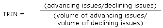
ARMS Index (TRIN Indicator) - $TRNN (NYSE), $TRNQ(NASDAQ)

                       Courtesy Investopaedia.com

A ratio of 1 means the market is in balance; above 1 indicates that more volume is moving into declining  and below 1 indicates that more volume is moving into advancing stocks. This indicator was developed by Richard Arms.

These are two ticker symbols within the FastTrack database.

Ulcer Index

Martin & McCann's book entitled "The Investor's Guide to Fidelity Mutual Funds" originated the Ulcer Index. Standard Deviation is increased by both gains and losses in portfolio value, yet a real investor is only disconcerted by the downside. Rapid increases in price create profits, not risk. Standard Deviation also does not distinguish between randomly occurring gains and losses and very long sequences of losses. Clearly a risk measure is highly desirable that addresses these deficiencies.

Source: Brian Stocks "FastTools v2.07 for FastTrack"

The Ulcer Index is obtained as follows:

Every day, determine the % amount 'R' that a mutual fund is below it's highest previous value. Calculate a running total of R-squared. Then divide this product by N, the total number of days in the period and take the square root of the quotient to obtain UI. The lower the Ulcer Index the easier an investment will be to live with and the less troubling it will be on the down days.

Ulcer Index = SquareRoot((The Sum of all R˛ values) / N)

Note: This calculation is made for the period between the poles.

Ulcer Performance Index (UPI)

The Ulcer Performance Index is a very good measure of the Risk Adjusted Return of an investment. It measures how well an issue outperforms a  Low Risk Base compared with the amount of ulcers it gives you. The higher theUPI value, the better the investment.

The Ulcer Performance Index for an Issue is obtained as follows:
Subtract the Annual Return of a Low Risk Base Mutual Fund  from the Annual Return of Issue. Divide the result by Ulcer Index of Issue to get the UPI.

Ulcer Performance Index = (Annualized Return of Issue - Annualized Return of Low Risk Base) / Ulcer Index of Issue

This calculation is made for the period between the poles.

UPI and Sortino are calculations sort in the same order with very few exceptions.

 

Note this comparison of UPI and Sortino.

http://investexcel.net/ulcer-index/

Welles Wilder RSI (I Chart)

The RSI chart uses one adjustable parameter, P (The number of days averaged). The calculations are based on day-to-day changes in Adjusted Price.

Step 1: Calculate an initial RSI using a simple average:

    a. Calculate the Simple Average of the Positive changes in value and another Simple Average of Negative changes in value.
        Both for P number of days.
                                         
                                        AvgDwn = Sum Positive / P
                                        AvgUp = Sum Negative / P

    b. Calculate the initial RSI using the Simple Averages of the Positive and Negative changes (This will be the RSI value for day P).
                                         
                                        Initial RSI = 100 - [ 100 / ( 1 + ( AvgUp / AvgDwn ) ) ]

Step 2: Calculate the remaining AvgUp and AvgDwn values  using an Exponential Average for Days > P

    a. AvgUp = [(Previous AvgUp * (P-1)) + Today's Negative Change (if there is one)]  / P

    b.  AvgDwn = [(Previous AvgDwn * (P-1)) + Today's Positive Change (is there is one)]  / P

Step 3: Calculate the RSI for Days < P

                RSI  = 100 - [ 100 / ( 1 + (AvgUp / AvgDwn) ) ]

FastTrack sets any value of RSI that is less than 1 to 1. This is unique to FastTrack and has no impact on the practical interpretation of the chart.

Yield

In the spreadsheet column , Yield is computed for the period between the poles as follows

Yield = TotalIncome / LDPrice Price

where

TotalIncome: LDPrice: Shares:

The total of income distributions of all types, adjusted for reinvestments. This total is reported on the Chart Tab. See Note. Last Day's actual closing (not dividend-adjusted) price The number of shares held on the last day. On first day, one share is held. The number of shares held on the last day is reported on the Chart Tab. See Note.

Yield1Y

In the spreadsheet column and on the Chart Tab's pole dates label, Yield1Y is computed  from the rightmost end of the chart back one year without regard to pole position or chart width.

Yield1Y = TotIncome / (FDPrice + TotCapGains)

where

TotalIncome: FDPrice: TotCapCains:

The total of income distributions of all types, adjusted for reinvestments. See Note. First Day's actual closing price (not dividend-adjusted) price Total capital gains paid during the year.

Morningstar says

"Investors who want to know the yield they actually received over the past year should look at a fund's distributed yield. This is the rate used by many financial publications, including Morningstar. It takes into account all dividends paid out over the previous 12 months and divides that figure by the sum of the fund's NAV and its capital gain distributions. It is essentially a historical yield and is good for comparing the dividends paid out by different funds."

Note: When the Chart Tab's Dashed Pole is placed on the chart's last date, the Pole Label displays the Total Income paid for the period displayed, adjusted for dividends. This is more than the sum of the per share dividends paid when there are multiple distribution days in the year. Each distribution purchases additional shares which then pay out slightly more when the next distribution occurs because, now, more than one share is held.  

Weird Numbers

It is normal that not all chart numbers in the printed manual or displayed in help will match what you see on your screen.

FastTrack Isn't Perfect  . . .  Yet

One reason for chart differences is that no known source of mutual issue data is perfect, not even FastTrack. When we discover that our data is incorrect we transmit changes to all users during their next download. This obviously will change numbers on the screen as compared to the static examples in the help.

Money Market funds are a special case. We distribute the dividends on a daily basis (Starting December 2008 in FT4Web 3.67). For the current month we distribute last month's dividend daily. When the actual dividend becomes available, the gain of the preceding month is recalculated. Thus, the returns that include the last month of money market gains will shift slightly when the next dividend posts. You will note that the money market daily lines still show closing prices of 1.00 for each day although the line rises slightly each day. If you want to see the adjusted values actually being charted, right-click the chart and select "Adjusted Close"

Total Return Chart

Cor=   is dependent on the data of the red line and the green line. If that data has been changed or if distributions have been added/changed for either line, then these values may change. Values may differ even when the Ru = and Ann= values remain constant. Ru = and Ann= are dependent on end point price and intervening distributions. Changes in Ru = and Ann= often reflect revised distributions. End points and "between the poles" Prices and distributions may affect Cor=. These values may change even when Ru = and Ann= are constant.

Indicator Charts

Aside from revised data as discussed above, indicators include other factors that can make chart numbers change. Over the evolution of FastTrack, the algorithms used in the indicators change.

• AccuTrack was revised to have two parameters instead of one.
• Stochastics were revised to improve computation speed.
• MACD and Moving average were revised to remove bogus whipsaws at the start of the data . . . and there have been many other changes between revisions.

All these type of changes can affect all or one of the values including Rsk=, S/Y=, Mr=, and Tr=.

Adjusted Return Charts (J and 2)

The J chart depends on the red and green lines. The 2 charts depends of the red and  2MM= issue. Also, the settings of  Trading Delay in the Parameters and the check box "Show White Line" option in the parameters.

Ra Computation WorkSheet

To compute the return for a period with Trading delays set to 0

Start filling in the second line

1. Right-click the chart and select adjusted prices. This means you will not have to deal with distributions. If you want to deal with distributions see the Distribution Worksheet.
2. Place the Dashed Pole on a first day of the period. Record the starting day's CP= where "1st price" is shown on the second line of the table.. Note that if the J or 2 chart performance values are green then use the T Chart's green CP= . If red, then use the T Chart's red CP= 
3. Move the Dashed Pole to the last day of the period. This would usually the day of the next signal. Record the proper colored CP= as the "last price" on the second line of the table.

Continue on the third and subsequent lines

1. In StartNAV enter the prior End NAV. 
2. Move the Dashed Pole to the end of the period (should have a signal tic on it). Record the End NAV.
3. Compute the Gain 
   (1.0 +  (End NAV-Start NAV)/Start NAV)
   This should equal the proper color T Chart's BP= value when the poles are placed on the Start and End. .
4. Multiply Gain and the "Ending Shares" from the line. Place the product in the "Ending shares" column.
5. Multiply Gain and the "Assets" on the current line. Place the product in the "Assets" column.
6. Compute the "Total Return" using the formula
   (Total Return from line above) * (1.0 + Gain)
   Enter the product in the "Total Return" column 

Finally, take the last Total Return and subtract 1 and multiply by 100. This is the percent gain that should be shown in the J Chart performance values as Adj=.

If your Trading Delay is NOT set to 0, then you must offset the poles by the appropriate number of days to match the FT4Web's Ra= values.

Yellow and Purple Values

We cover these values as a separate subject. Yellow values occur throughout indicators and various charts. They change a great deal because yellow values are based Adjusted Prices (P Chart's yellow and purple values are actually readjusted back to a quasi-unadjusted value that makes the value relate to your brokerage statements and the prices printed in the paper daily.)

There is a detailed description of Adjusted Price  including a worksheet that shows how to compute Adjusted Price  .  .  . so we won't go into a lot of detail here.

The most salient aspect of Adjusted Price is that whenever there is a new distribution posted in the database, previous yellow values change. Therefore, except for the P Chart, do not expect ANY printed yellow or purple values to agree with what you see on the screen. HOWEVER, you should expect that the percentage change between any two days will stay the same except when red line, green line, or distribution data has been changed.

Exponential Moving Average

The goal is to produce a smoothed line through exponential moving averaging.

1. Calculate a smoothing factor (SFactor) derived from a parameter value (typically a number of days) . This factor is a constant throughout the averaging process.
   
   SFactor = 2 / (Parameter + 1)
    
2. Each day's moving average value (MA) is computed as follows,
   
   MA = ( Price * SFactor ) + ( prior MA * (1 -  SFactor) )
   
   On the first day, MA is set to the first day's Price. The MA is carried forward to the next day to be used as the prior MA in the formula.

Relative Standard Deviation Spreadsheet Column (RelSD)

This column show the result of dividing each issue's SD value by its Relevant Index SD. 

RelSD should hover around a value of 1.0 assuming that the Relevant Index is properly matched. This is a calculation in which the Standard Deviation of each member of a sample is divided by the average SD of all members. This calculation is a compromise to serve the same function, we recognize that the result is not precisely the same as is typical in a relative SD computation.

In general, conservative investors would want a portfolio of issues that have a RelSD<1. Aggressive investors would want a portfolio of issues with RelSD>1.

For issues that have no Relevant index, the SD of the green line is used.